- Introduction
- Terminal and Initial objects
- Products and Coproducts
- Pullbacks and Pushouts
- Natural transformations
- Representable functors and the Yoneda Lemma
- Adjunctions (part 1)
- Monads
- Adjunctions and monads
- String diagrams
- Pipe cleaners
- General Limits and Colimits
- Slice and comma categories
- Coequalisers
- Monoid objects
- 2-categories
- Eckmann-Hilton
- Distributive laws
- Group Objects and Hopf Algebras
- Ends
- Adjunctions from morphisms
- Double Categories
- Spans
- Multicategories
- Metric Spaces and Enriched Categories
Introduction
In an attempt to solidify and extend my knowledge of category theory, I have been working my way through the excellent series of category theory lectures posted on Youtube by Eugenia Cheng and Simon Willerton, aka the Catsters.
Edsko de Vries used to have a listing of the videos, but it is no longer available. After wresting a copy from a Google cache, I began working my way through the videos, but soon discovered that Edsko’s list was organized by subject, not topologically sorted. So I started making my own list, and have put it up here in the hopes that it may be useful to others. Suggestions, corrections, improvements, etc. are of course welcome!
As far as possible I have tried to arrange the order so that each video only depends on concepts from earlier ones. Along with each video you can also find my cryptic notes; I make no guarantee that they will be useful to anyone (even me!), but hopefully they will at least give you an idea of what is in each video. (For some of the earlier videos I didn’t take notes, so I have just copied the description from YouTube.)
I have a goal to watch two videos per week (at which rate it will take me about nine months to watch all of them); I will keep this list updated with new video links and notes as I go.
Terminal and Initial objects
Terminal and initial objects 1
- Definition and examples of terminal objects
- Sketch of proof that terminal objects are unique up to unique isomorphism
Terminal and initial objects 2
- Proof that terminal objects are unique
- Examples of categories without terminal objects
Terminal and initial objects 3
- Definition and examples of initial objects
Products and Coproducts
Products and coproducts 1
- Definition of products
- Example: cartesian product of sets
and
as two (isomorphic) products
- Uniqueness up to unique isomorphism
Products and coproducts 2
- More on uniqueness up to unique isomorphism
- Examples and non-examples of products
Products and coproducts 3
- Definition and example of coproduct
Products and coproducts 4
- Definition of the morphisms
and
- The diagonal
- Products with the terminal object

Pullbacks and Pushouts
Pullbacks and pushouts 1
- Definition of pullback
- Example: pullbacks in
Pullbacks and pushouts 2
- Definition of pushouts
- Example: pushouts in
- Pullback/pushout example of intersection/union of sets
Natural transformations
Natural transformations 1
- Definition of natural transformations.
- Naturality squares.
- Intuition about natural transformations based on homotopy.
- Alternative definition of natural transformation analogous to usual homotopy definition: a natural transformation is a functor
where
is the “categorical interval”, i.e. the two-object category with a single nontrivial morphism.
Natural transformations 2
- Vertical composition of natural transformations.
- Functor categories.
- Horizontal composition of natural transformations
- Note there are two ways to define horizontal composition, and they are equal by naturality.
Natural transformations 3
- Whiskering (though they don’t call it that yet).
- Horizontal composition as vertical composition of two whiskerings (in two different ways, which are equal by naturality).
- Interchange law: proof by commutativity of whiskering.
Natural transformations 3A
- Define terminology “whiskering”.
- Note vertical composition of “right-whiskered fish” works because of functoriality (of functor we whiskered by).
- Vertical composition of “left-whiskered fish” comes by definition of vectical composition for natural transformations.
- So in the end, interchange depends on three things: definition of vertical composition; functoriality; naturality.
Representable functors and the Yoneda Lemma
Representables and Yoneda 1
- Definition of representable functors (co- or contravariant): those which are naturally isomorphic to
or
for some
.
- Contravariant:
;
.
- Covariant:
;
.
- Contravariant:
- Is there a functor
? Yes, the Yoneda embedding
:
, where
is postcomposition with
.
is a natural transformation; its component at
has type
. Postcomposing an arrow in
with
yields an arrow in
.

Representables and Yoneda 2
- Proof that Yoneda embedding
sends morphisms
Representables and Yoneda 3
- Look at natural transformations from
. Big idea: such natural transformations
are entirely determined by where
sends
.
- Yoneda lemma:
(natural in
is isomorphic to the hom-set of natural transformations between
Adjunctions (part 1)
Adjunctions 1
- Given categories
and
and functors
and
, we have the following situations:
- Isomorphism:
,
- Equivalence:
,
- Adjunction:
,
So we can think of an adjunction as a “weaker sort of equivalence”.
- Isomorphism:
and
are subject to triangle identities:
is the identity, and similarly for
.
- These laws can be expressed as commuting diagrams of 2-cells: draw


Adjunctions 2
- Alternate definition of adjunction
: an isomorphism
natural in
- What “natural in
- Hint: sending identity morphisms across the iso gives us
Adjunctions 4
- Note: Adjunctions 4, not 3, follows on to 2.
- Given: an isomorphism
which is natural in
- Notation: write application of the isomorphism as an overbar.
- Construct the two squares implied by naturality. Follow them each around in both directions (since they involve a natural isomorphism) to get four equations in total governing how the iso interacts.
- Define
Monads
Monads 1
- Monads give us a way to talk about algebraic theories (monoids, categories, groups, etc.).
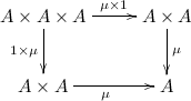
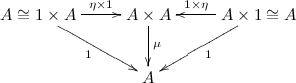
- Definition of a monad:
- Functor
- “unit”
- “multiplication”
- with unit and associativity laws.
- Functor
- Note what is meant by a commutative diagram of natural transformations
- Example: monad for monoids (aka the list monad)
, maps a set
is concatenation
- Note, unit and associativity for monad is different than unit and associativity of monoids, which has already been encoded in the definition of
.


Monads 2
- Proof that the list monad (“monad for monoids”) is in fact a monad
- Example: monad for small categories
, category of graphs
- With only one object, this reduces to the monad for monoids.
- Proof of monads laws is basically the same as for the list monad.
Monads 3
- Algebras for monads. Monads are supposed to be like algebraic theories; algebras are models.
- An algebra for a monad
is an object
(the “underlying object”) equipped with an “action”
, satisfying the “obvious” axioms (
must interact “sensibly” with
- Example:
,
- An algebra is a set
- First axiom says
- Other axiom is essentially associativity.
- That is, algebras for the list monad are monoids.
- An algebra is a set
- Example for monad of categories (from last time) works the same way.


Monads 3A
More on monoids as monad algebras of the list monad.
- Given a monad algebra
, construct the monoid:
- whose underlying set is
.
- whose underlying set is
- The monad algebra law for
- Identity and associativity laws for the monoid come from the other monad algebra law, saying how
![a \cdot b = \theta [a,b]](https://s0.wp.com/latex.php?latex=a+%5Ccdot+b+%3D+%5Ctheta+%5Ba%2Cb%5D&bg=ffffff&fg=333333&s=0&c=20201002)
Monads 4
Monad algebras form a category (called 
-
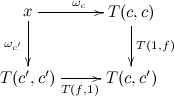
Given two monad algebras
and
, a morphism between them consists of a morphism of underlying objects,
, such that the obvious square commutes.
-
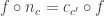
Example. List monad again.
. A morphism of monoids is a function
. See how this equation arises from the commuting square for monad morphisms, by starting with a 2-element list in upper left and following it around.
-
Given a particular mathematical theory, can it be expressed as the category of algebras for some monad? I.e. given a category
-
But this is still an interesting question, more or less the question of “monadicity”. Category
Adjunctions and monads
Adjunctions 3
- Note: depends on monads.
- Examples of adjunctions:
- between the category of sets and the category of monoids:
- similarly between category of graphs and category
of (small) categories.
In general, free functors are left adjoint to forgetful functors. (How to remember the direction: “left” has four letters, just like “free”.)
- between the category of sets and the category of monoids:
- Every adjunction
gives rise to a monad
. Check monad laws:
- Monad triangle laws are just adjunction triangle laws with extra
or
- Monad associativity law is naturalty for
- Monad triangle laws are just adjunction triangle laws with extra

Adjunctions 5
“Every monad comes from an adjunction via its category of algebras.”
Last time we showed every adjunction gives rise to a monad. What about the converse?
Answer: yes. In fact, given a monad, there is an entire category of adjunctions which give rise to it, which always has initial and terminal objects: these are the constructions found by Kleisli and by Eilenberg-Moore, respectively. Intuitively, any other adjunction giving rise to the monad can be described by the morphisms between it and the Kleisli and Eilenberg-Moore constructions.
Let
-
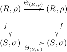
Terminal solution (Eilenberg-Moore): consider category
. We construct an adjunction
. (Intuition:
“freely” constructs a
“forgets” the algebra structure.)
-
.
-
What about
. Then evaluation map is
. Need to check that this definition of
-
Now define a unit and counit.
is just the
is an algebra morphism from the free algebra on
) to
: in fact,
-
Prove triangle laws for
-
Adjunctions 6
This time, initial solution to “does a monad give rise to any adjunctions”: Kleisli.
- The Kleisli category for a monad
or
- Objects: objects of
- Morphisms:
.
- Composition: given
and
, produce
.
- Identity:
.
- Category axioms come from monad axioms. Associativity comes from associativity and naturality of
- Objects: objects of
-
Intuition: this is the category of free algebras:
is equivalent, under the adjunction, to
, morphism between free algebras.
-
Note, for the Eilenberg-Moore category (last time) it was complicated to define the objects and simple to define the morphisms. For Kleisli, it’s the other way around. “Conservation of complicatedness.”
Adjunctions 7
The adjunction that comes from the Kleisli category, giving rise to the original monad
Again, let 


sends objects to “free algebras”
- Identity on objects.
- On morphisms, sends
(equivalently
).
sends a “free algebra” to its “underlying object”
- Sends
- Sends
.
- Sends
- Unit and counit
we can take as the
we can take to be id.
- Adjunction laws come down to monad laws (left to viewer).
Given a monad 
Question of monadicity: given an adjunction 
String diagrams
String diagrams 1
Way of notating natural transformations and functors. Poincare dual: 0D things (points, i.e. categories) become 2D (regions), 1D things (lines, i.e. functors) stay 1D, 2D things (cells, i.e. natural transformations) become 0D.
String diagrams should be read right-left and bottom-top.
Horizontal and vertical composition of NTs correspond to horizontal and vertical juxtaposition of string diagrams.
Can leave out vertical lines corresponding to identity functor.
String diagrams 2
Recall the interchange law, which says that vertical and horizontal composition of natural transformations commute. This guarantees that string diagrams are well-defined, since the diagram doesn’t specify which happens first.
Whiskering is represented in string diagrams by horizontally adjoining a straight vertical line.
String diagrams 3
Given an adjunction 

String diagrams 4
Monads in string diagrams. Draw
String diagrams 5
Seeing how monads arise from adjunctions, using string diagrams.
Pipe cleaners
These are presented without any commentary or explanation that I can find. Each of the below videos just presents a 3D structure made out of pipe cleaners with no explanation. Maybe there is some other catsters video that presents a motivation or explanation for these; if I find it I will update the notes here. I can see that it might have something to do with string diagrams, and that you can make categories out of these sorts of topological structures (e.g. with gluing as composition) but otherwise I have no clue what this is about.
- Open-closed cobordisms 1: http://youtu.be/Jb1ZHLXBMy4
- Open-closed cobordisms 2 (“zig-zag-ator”): http://youtu.be/zQMhXy1-YNM
- Open-closed cobordisms 3 (“cut-off pair of pants”): http://youtu.be/_raQJYpEnU8
There is also:
- Klein bottle: https://www.youtube.com/watch?v=kteH2ZBW9Lg
This is a nice 5-minute presentation about Klein bottles, complete with pipe cleaner model. Though it seems to have little to do with category theory.
Also also:
This has nothing to do with either pipe cleaners or category theory, but it is midly amusing.
General Limits and Colimits
General limits and colimits 1
Defining limits in general, informally.
- The thing we take a limit of is called a diagram (a collection of objects and morphisms). A limit of a diagram is a universal cone.
- A cone over a diagram is an object (vertex) together with morphisms (projection maps) to all objects in the diagram, such that all triangles commute.
- Universal cone is the “best” one, through which all other cones factor, i.e. there is a unique morphism from the vertex of one to the other such that all the relevant triangles commute.
General limits and colimits 2
Examples of limits.
- Terminal objects: limit over the empty diagram.
- Products: limit over discrete diagram on two objects.
- Pullback: limit over a “cospan”, i.e. a diagram like
. Note that we usually ignore the edge of the cone to
.
- Equalizer: limit over a parallel pair of arrows.
General limits and colimits 3
- Note: requires natural transformations.
- Formal definitions of:
- Diagram (functor from an index category)
- Cone (natural transformation from constant functor to diagram).
General limits and colimits 4
- Requires Yoneda.
-
Formal definition of a limit: given a diagram
, a limit for
together with a family of isomorphisms
natural in
. I.e. a natural correspondence between morphisms
(the “factorization” from one cone to another) and morphisms (i.e. natural transformations) from
to
(i.e. cones over
-
If we set
then
etc. In particular
corresponds to some cone, which is THE universal cone. The Yoneda lemma says (?) that the entire natural isomorphism is determined by this one piece of data (where
goes). Note that both
and
are functors
. The Yoneda lemma says that a natural transformation from
to
— i.e. a cone with vertex
-
The universality of this cone apparently comes from naturality.
General limits and colimits 5
- Requires adjunctions.
- Notation for limits. Categories that “have all limits (of a given shape)”.
- The natural isomorphism defining a limit can be seen as an adjunction
where
, and
is the functor that takes a diagram and produces its limit.
- Claim: this is an adjunction if
is actually a functor.
General limits and colimits 6
Colimits using the same general formulation. “Just dualize everything”.
-
Cocone (“cone under the diagram”) is an object with morphisms from the objects in the diagram such that everything commutes.
-
Universal cocone: for any other cocone, there is a unique morphism from the universal cocone to the other cone which makes everything commute. Note it has to go that direction since the universal cocone is supposed to be a “factor” of other cocones.
-
In Eugenia’s opinion the word “cocone” is stupid.
-
More generally: natural isomorphism between cocones and morphisms.
. Limits in
, and vice versa.
-
All limits are terminal objects in a category of cones (and colimits are initial objects).
-
Since terminal objects are initial objects in
Slice and comma categories
Slice and comma categories 1
Slice category. Given a category 

- Objects are pairs
where
.
- Morphisms from
are morphisms
in
Coslice category, or “slice under” category 

-
If
,
. (Dually,
.)
-
Products in
Slice and comma categories 2
Comma categories are a generalization of slice categories. Fix a functor 

- Objects: pairs
. Image of some object under
- Morphisms are morphisms
makes the relevant diagram commute.
Of course we can dualize, 
Apparently comma categories give us nice ways to talk about adjunctions.
Let’s generalize even more! Fix the functor 
- Objects: triple
.
- Morphism
is a pair of morphisms
and
such that the relevant square commutes.
Can also dualize, 
An even further generalization! Start with two functors 

- Objects: triples
.
- Morphisms: obvious generalization.
In fact, all of these constructions are universal and can be seen as limits/colimits from the right point of view. “Next time”. (?)
Coequalisers
Coequalisers 1
Coequalisers are a colimit. Show up all over the place. Give us quotients and equivalence relations. Also tell us about monadicity (given an adjunction, is it a monadic one?).
Definition: a coequaliser is a colimit of a diagram consisting of two parallel arrows.
More specifically, given 


-
Example: in
: coequaliser of
, where
is the equivalence relation generated by
for all
.
-
Conversely, we can start with an equivalence relation and build it using a coequaliser. Given: an equivalence relation
. Note we have
. Coequaliser is equivalence classes of
.
Coequalisers 2
Quotient groups as coequalisers. Consider a group 


Let’s see why. Suppose we have another group 


Notation: 
![[g] = gH](https://s0.wp.com/latex.php?latex=%5Bg%5D+%3D+gH&bg=ffffff&fg=333333&s=0&c=20201002)


![[g]](https://s0.wp.com/latex.php?latex=%5Bg%5D&bg=ffffff&fg=333333&s=0&c=20201002)


![[g_1] [g_2] = [g_1 g_2]](https://s0.wp.com/latex.php?latex=%5Bg_1%5D+%5Bg_2%5D+%3D+%5Bg_1+g_2%5D&bg=ffffff&fg=333333&s=0&c=20201002)
Monoid objects
Monoid objects 1
Idea: take the definition of monoids from
- A monoid is:
- A set
- A binary operation
on
- A unit
- Associativity:
- Identity:
- A set


Now let’s reexpress this categorically in
- A monoid (take 2) is:
- An object
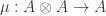
- A morphism
(note we use Cartesian product structure of
- A morphism
- A commutative diagram
- A commutative diagram
- An object


Now we take the definition and port it to any monoidal category.
- A monoid object in a monoidal category
- An object
- A morphism
- A morphism
- A commutative diagram
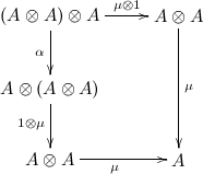
- A commutative diagram
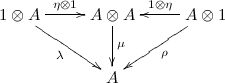
- An object

Monoid objects 2
Today: monoid object in the category of monoids is a commutative monoid.
Note first the category of monoids is itself monoidal under Cartesian product. That is, given two monoids 


Now, what is a monoid object in 
- An object
, i.e. a monoid
- Monoid morphisms
and
- …satisfying unit and associativity laws.


Monoid object is also required to satisfy unital and associativity laws, but we can already deduce those from Eckmann-Hilton.
2-categories
2-categories 1
Generalization of categories: not just objects and morphisms, but also (2-)morphisms between the (1-)morphisms. Primordial example: categories, functors, and natural transformations.
Note: today, strict 2-categories, i.e. everything will hold on the nose rather than up to isomorphism. A bit immoral of us. [If we let things be a bit looser we get bicategories?]
Recall: a (small) category
- A set
of objects
- for all
, a set
of morphisms
equipped with
- identities: for all
a function
- composition: for all
, a composition function
.
- unit and associativity laws.
To make this into a 2-category, we take the set of morphisms and categorify it. That turns some of the above functions into functors. Thus, a 
- a category
- a functor
for each
- a composition functor
.
- etc.

(Note: why not turn the set of objects into a category? That’s a good question. Turns out we would get something different.)
Let’s unravel this a bit. If 
We also have the composition functor
Next time: how functoriality gives us the interchange law.
2-categories 2
Interchange in a 2-category comes from functoriality of the composition functor. The key is to remain calm.
The functor is
Eckmann-Hilton
Eckmann-Hilton 1
NOTE: There seems to be no catsters video actually explaining what a “bicategory” is. According to the nlab it is a weaker version of a 2-category, where certain things are required to hold only up to coherent isomorphism rather than on the nose.
Eckmann-Hilton argument. Originally used to show all higher homotopy groups are Abelian. We can use it for other things, e.g.
- A bicategory with only one 0-cell and one 1-cell is a commutative monoid.
- A monoid object in the monoidal category of monoids is a commutative monoid. (waaaat)
Idea: given a set with two unital binary operations, they are exactly the same, and commutative — as long as the operations interact in a certain coherent way.
Given a set with two binary operations 
- one of them distributes over the other, i.e.
,
then 
Geometric intuition:
Proof: use the “Eckmann-Hilton clock”. See video for pictures. Given e.g. 


In fact, it is not necessary to require that the two units are the same: it is implied by the interchange law. Left as an exercise.
Eckmann-Hilton 2
This time, show the interchange law implies the units are the same and associativity.
Let 


Example. A (small)
Bicategory case is a bit more complicated, since horizontal composition is not strictly unital. A bicategory with only one
Distributive laws
Distributive laws 1
Monads represent algebraic structure; a distributive law says when two algebraic structures interact with each other in a coherent way. Motivating example: multiplication and addition in a ring.
Let 


Example: 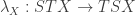


In fact we have constructed the free ring monad, 
If we start with a monoid and consider the free group on its underlying elements, we can define a product using distributivity; so the free group on a monoid is a group. Formally, the free group monad lifts to the category of monoids (?).
Distributive laws 2
More abstract story behind our favorite example: combining a group and a monoid to get a ring.
Note: distributive law (at least in this example) is definitely non-invertible: you can turn a product of sums into a sum of products, but you can’t necessarily go in the other direction.
Main result: A distributive law 

When is 

Distributive law is equivalent to a lift of
- An
; we want
. But we have
; precomposing with
-
Since
, a
to
This essentially says that an algebra for
-
An algebra for
. Clear that from a
with
to get an
to get a
Distributive laws 3 (aka Monads 6)
Recall that a monad is a functor together with some natural transformations; we can see this as a construction in the
Let
- a
- a
- a pair of
and

satisfying the usual monad axioms.
In fact, we get an entire
What is a morphism of monads? A monad functor 
- a
- a
(Note, this is not backwards! This is what we will need to map algebras of the firs monad to algebras of the second.)

satisfying the axioms:


A monad transformation (i.e. a
- a
, satisfying
(something like that, see pasting diagrams of
Distributive laws 4
Distributive laws, even more formally!
Consider the 
Recall that a monad in an arbitrary
- A
.
- A
, that is, a functor
and
- Axioms on
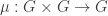
Summarizing more concisely/informally, a monad in
- A
- A pair of monads
- A distributive law
Consider the map 

The multiplication has type 

Group Objects and Hopf Algebras
Group Objects and Hopf Algebras 1
Take the idea of a group and develop it categorically, first in the category of sets and then transport it into other categories (though it may not be completely obvious what properties of
A group is of course a set
So a group is:
- an object
- a multiplication morphism
- an inverse morphism
- a unit morphism
(i.e. “universal element”)


together with axioms expressed as commutative diagrams:
(note to be pedantic we also need to use
and
)


where 


Group Objects and Hopf Algebras 2
Note just 
Recall
In fact, every set 
- a comultiplication
- a counit
- satisfying coassociativity and counit axioms.


And note we used
Group Objects and Hopf Algebras 3
The definition given last time won’t work in general for any monoidal category, but it does work for any Cartesian category (that is, monoidal categories where the monoidal operation is categorical product). Examples of Cartesian categories, in which it therefore makes sense to have group objects, include:
(category of topological spaces, with Cartesian product toplogy)
(cat. of smooth manifolds?)
(groups)
Let’s see what a group object looks like in each of these examples.
- In
- In
- In
- In
- In
What about non-Cartesian monoidal categories? Simplest example is 
![V \otimes W = \{ \sum_t \alpha_t (v_t \otimes w_t) \mid v_t \in V, w\_t \in W \} / [(\alpha_1 v_1 + \alpha_2 v_2) \otimes w \sim \alpha_1 (v_1 \otimes w) + \alpha_2(v_2 \otimes w) \text{ and symmetrically}]](https://s0.wp.com/latex.php?latex=V+%5Cotimes+W+%3D+%5C%7B+%5Csum_t+%5Calpha_t+%28v_t+%5Cotimes+w_t%29+%5Cmid+v_t+%5Cin+V%2C+w%5C_t+%5Cin+W+%5C%7D+%2F+%5B%28%5Calpha_1+v_1+%2B+%5Calpha_2+v_2%29+%5Cotimes+w+%5Csim+%5Calpha_1+%28v_1+%5Cotimes+w%29+%2B+%5Calpha_2%28v_2+%5Cotimes+w%29+%5Ctext%7B+and+symmetrically%7D%5D&bg=ffffff&fg=333333&s=0&c=20201002)
Suppose 


The point is that 

Group Objects and Hopf Algebras 4
We still want to be able to define group objects in monoidal categories which are not Cartesian.
Recall: if we have a monoidal category 

Notation: in 
A Hopf algebra is a group object in a general monoidal (tensor) category. Details next time.
Group Objects and Hopf Algebras 5
A Hopf algebra 
- comonoid
and
- monoid
and
- “antipode” or inverse


(See video for string diagrams.) Note the monoid and comonoid also need to be “compatible”: this is where the braidedness comes in. In particular 
Lemma: suppose 


Can then write down what it means for
Group Objects and Hopf Algebras 6
String diagram showing comonoid
There seems to be some asymmetry: monoid + comonoid + monoid must be comonoid morphisms. But it’s the same to say that the comonoid must be monoid morphisms.
Ends
Ends 1
Given a functor 

Ends are not as common as coends (and perhaps not as intuitive?). Two particular places where ends do show up:
- natural transformations (especially in enriched setting; see Ends 2)
- reconstruction theorems (recover an algebra from category of its representations, i.e. Tannaka reconstruction, see Ends 3)
Definition:
- A wedge
consists of
- an object
- a family of
for all
- such that for all
the obvious square with vertices
,
,
, and
commutes. (Dinaturality/extranaturality.)
- This is in some sense a generalization of a cone.
- an object
-
An end is a universal wedge, i.e. a wedge
such that if
then there exists a unique morphism
through which the components of

Note we write the object 
Ends 2
Simple example of an end: 
- some
- for each
a function
- such that
we have
.


That is, for every 


Note this goes in the other direction too, that is, a wedge 

Ends 3
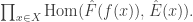
More examples. First, straightforward generalization: given functors 


(Proof is just a small generalization of the proof in Ends 2, left as exercise.) Useful in an enriched context, can use this end to construct an object of natural transformations instead of a set.
Another example, “baby Tannaka reconstruction” (see Tannaka duality and reconstruction theorem on nlab).
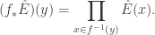
is the forgetful functor.
- Result:
. (In general, natural transformations over forgetful functor reconstructs algebraic objects.)
Proof (application of Yoneda):
- Let
- An
. Morphisms
are just functions
which commute with the actions (“equivariant maps”).
- Note
- Consider the
(“left-regular representation of
- Define
by
.
- Note
determines
. In fact
.
- Thus
.
- Consider the
- So
, and by (co-?)Yoneda, this is just
.
Ends 4
Combine some of the previous examples. Recall
(Ends 2)
(Ends 3)
What happens if we combine these two results? First, look at the end from last time:
- Let
be a natural transformation on
is a function
, such that
commutes with the underlying function of any equivariant map, i.e.

- As we showed last time,
for some
.
- Note
Now look at the end of the bare hom-functor in the category of
-
Now if
, we have
-
What’s the difference?
is now a family of equivariant maps. But note equivariant maps are determined by their underlying function. So any diagram of this form implies one of the previous form; the only thing we’ve added is that
.
i.e. we’re picking out some subset of
we know
for some
; which
-
Consider the left-regular representation
again. Then we know
is just left-multiplication by some
. But it has to commute with equivariant maps; picking the action on the particular element
that is,
, i.e.
.
-
So we conclude
.

Adjunctions from morphisms
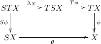
Adjunctions from morphisms 1
General phenomenon: associate some category 
- In representation theory, to a group or algebra we associate a category of modules or representations.
- In algebraic topology, to a space
(category of “bundles”?)
- In algebraic geometry, to an algebraic variety associate the category of sheaves.
- In logic, to a set of terms associate a category of subsets (predicates) over the terms.
- In analysis, to a metric space
.
Question: if we have a morphism 

We often get some sort of “pullback” functor 

We also get various “pushforwards” 
This is the beginning of the story of “Grothendieck’s 6 operations”. Lots of similar structure arises in all these different areas.
Adjunctions from morphisms 2
Baby examples of some particular adjunctions (in generality, they show up in Grothendieck’s 6 operations, Frobenius reciprocity, …). Idea: start with (e.g.) sets; to each set associate a category; to each morphism between sets we will get functors between the categories.
- To the set
.
- Think of the objects of this slice category,
, as “bundles over
- Another way to think of this is as a functor
(considering
- Think of the objects of this slice category,
-
There is actually an equivalence of categories
.
-
What about maps between sets? e.g.
,
, and
, with
. Details in the next lecture.
Adjunctions from morphisms 3
-
Given
: to each
we associate the fiber of
. That is,
-
Now for the other direction. Idea: given a bundle over
, for each
we have a set
which are sent to that
by

(Foreshadowing: taking the disjoint union gives us another adjoint.)
Adjunctions from morphisms 4
Proof of the adjunction 
-
Notation:
instead of
or
-
Such hom-sets are a collection of maps between fibers, one for each base point.
-
So we have
.
-
We can partition
.
-
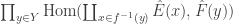
A product of hom-sets is isomorphic to a hom-set into a product (i.e.
), so this is equal to
.
-
By definition of
, this is
.
-
Finally, by definition of
, this is
.
-
Of course technically we would need to show naturality as well, but this is the basic idea.

Adjunctions from morphisms 5
Last time, we proved an adjunction

In fact, we showed that both are isomorphic to
i.e. given some 

Using the same trick as last time, this is equivalent to 
(since 
This gives us a left adjoint 

Remark: note that if we view bundles over 
Double Categories
Double Categories
Internal categories in 

If 


are
are “vertical
What about composition? Note
Note if all vertical
Spans
Spans 1
NOTE: There seems to be no catsters video actually explaining what a “bicategory” is. According to the nlab it is a weaker version of a 2-category, where certain things are required to hold only up to coherent isomorphism rather than on the nose.
Let 
are spans
.
-
is a morphism
which makes things commute.
-
- Vertical
-
Horizontal
Can check all the axioms etc.
Now, note monads can be constructed inside any bicategory, and are given by
- a
- a
It turns out that monads in 
Spans 2
Monads in 
We have
- a
.
- a
(idea is that
will be the set of morphisms, and
- a
such that
, that is,
- a
.
is given by a pullback: a pair of morphisms such that the target of the first equals the source of the second, i.e. a composable pair.
And of course there are some monad laws which amount to the category laws.
More generally, monads in
- an “objects object”
- a “morphisms object”
- source and target maps
- identities and composition as before.

Multicategories
Multicategories 1
Like categories, but morphisms have multiple objects as their source.
A (small) multicategory
- a set of objects,
- For all
, a set
of morphisms.
- Composition: a morphism with
inputs can be composed with
- Identity morphisms, with just one input and output.

Note that one can have a morphism with no inputs.
This can all be expressed nicely using the “free monoid monad” (i.e. list monad). Let
Make a bicategory of
.
- Composition uses pullbacks and multiplication of
- Identity is
using
.
Bicategory axioms follow from monad laws for
Multicategories 2
We’ve seen that monads in Span are categories.
We’ve seen a category of 
Recall that
A monad in
- a set
- a
is a
(picking out the sequence of input objects) and from
- a
- a
Key point: we can actually do this with other monads
Metric Spaces and Enriched Categories
Metric Spaces and Enriched Categories 1
Idea due to Lawvere. A metric 
- Triangle inequality:


Compare to the data for a category, written in a slightly funny way:

These look remarkably similar! In fact, they are both examples of enriched category. We’ll start with a normal category and show how to generalize it to an enriched category.
Let
- a collection
,
,
,
- …satisfying associativity and unit laws.


Important thing to note: composition and identity are morphisms in 
In particular, if 
- collection
as before
, i.e we don’t have hom-sets but hom-objects that live in the category
- The composition map is a morphism
in
- Identity morphisms are now given by a morphism
in
- …satisfying associativity and unit laws.
e.g. pick
What if we take 

Metric Spaces and Enriched Categories 2
Explains in more detail how categories enriched in 
- For each pair of objects we have a “Hom-object” which is a nonnegative real number. (“distance”)
- Composition is supposed to be a morphism
. But
is
is
- Identity morphisms are given by
, i.e. distance from
- Associativity and unit laws are vacuous.
This is actually a generalized metric space. More general than a metric space in several ways:
- Distance is not symmetric:
. This actually has many real-world models (e.g. time to go between towns in the Alps).
- We might have
for
.
- We allow “infinite” distances (???)
Now we can study metric spaces categorically.
Given two 
- a map
, and
- for all
,
(a morphism in
In the generalized metric setting, such a
Metric Spaces and Enriched Categories 3
Enriched natural transformations. There are actually various ways to generalize. Today: simple-minded version. Apparently if we generalize the notion of a set of natural transformations we get a slightly better definition—this will be covered in future videos. [editor’s note: to my knowledge no such future videos exist.]
Standard definition of a natural transformation 


Simple way around this: let 


e.g. if 

In the example we care about, 


So now we can say that
So, let 
- for all
.
- Big commuting diagram expressing naturality in the enriched setting (see the video).


Pingback: Catsters guide | blog :: Brent -> [String]
Hey, they started posting new videos too!
Only two videos per week? My reaction upon finding Casters was to binge watch. ;-0 It’s kind of nostalgic to see these again actually. Remember when youtube had 11 minute time limits?
Thanks! Have you or has anyone else made this sequence into Youtube playlist?
Thanks!
Excellent. Many thanks!
Hi, Brent! I keep returning to your casters guide — it is very useful.
I think you are missing a link to the second [Eckmann-Hilton video](https://www.youtube.com/watch?v=wnRqo7UHa-k)
You’re right, thanks for pointing that out! Fixed now.
I totally love you <3. Thank you very much for this.
Pingback: In praise of Beeminder | blog :: Brent -> [String]
Edsko de Vries list can now be found at http://simonwillerton.staff.shef.ac.uk/TheCatsters/ according to the Catsters channel About page.
Oh, thanks for the link!
list monad (“monad for monoids”) should be monad for _free_ monoids. And this is a general pattern: if there is a free-forgetful adjunction F -| U : C -> D involving categories of algebraic structures, then the category of algebras of the monad UF is equivalent to the category C.
More details see https://www.schoolofhaskell.com/user/dolio/many-roads-to-free-monads#algebras-of-a-monad
This is great, thanks. Are you aware of any resources that view Category Theory from a computational/algorithmic perspective? All the resources (like free books available on the subject) I have come across are too abstract for me.
Here are a few things off the top of my head. Not sure what counts as concrete enough for you — category theory is fairly abstract, after all! — but these do approach CT from a computational perspective:
Category Theory for Programmers, by Bartosz Milewski (available online at https://bartoszmilewski.com/2014/10/28/category-theory-for-programmers-the-preface/ or in dead tree form at http://www.lulu.com/shop/bartosz-milewski/category-theory-for-programmers/hardcover/product-23389988.html
Category Theory for Computing Science by Barr & Wells: http://www.math.mcgill.ca/triples/Barr-Wells-ctcs.pdf
Thanks much. The first link looks great. I have in the past gone through and solved problems up till generalized limits… and then got lost with adjoints and further. Even though I have taken a fair amount of graduate courses in abstract algebra I still find these difficult to follow. I guess I am asking if there is a computational viewpoint to these concepts in category theory. I am thinking of something like Burnside’s lemma in group theory and the entirely concrete application to counting in combinatorics. I don’t know if I am making much sense. Maybe types and programming is as concrete category theory will ever get :| … thanks!
No, you are making a lot of sense! Adjunctions in particular do come up *all the time* in computational contexts, and can definitely be thought about in a computational way. See https://hackage.haskell.org/package/adjunctions-4.3/docs/Data-Functor-Adjunction.html . An adjunction can be thought of as a sort of weakened bijection/isomorphism, where you don’t necessarily come back to where you started if you go across the adjunction and back. This kind of situation where two things are related/dual but not exactly isomorphic is very common. For example, abstract syntax trees and strings can be related by a parser/pretty-printer pair, but parsing and then pretty-printing may not be the identity. You may be interested in learning about Galois connections, which are a more specialized form of adjunction but have a lot of applications in computation (the example I gave above is actually a Galois connection). Adjunctions are also often used when doing formal equational reasoning about programs. See, e.g. http://www.cs.ox.ac.uk/ralf.hinze/LN.pdf . In fact that paper shows how most of the basic primitives in type theory/functional programming (product types, sum types, etc.) all ultimately come from adjunctions.
Yea, I had encountered Galois connections before I came across category theory. I had seen it in galois thoery and have also seen it in used in frequent itemset mining papers too many years ago! I’d definitely be interested in more applications of it though…. any links you have would be great!
I’ll have to give it more thought and dig around a bit, but I’m sure I can come up with some!
I would suggest moving Monoid objects down in the topological sort, because Monoid object 2 depends on Eckmann-Hilton.
Ah, thanks! But hmm, Eckmann-Hilton seems to mention monoid objects a bunch. Have we discovered a cycle?